from sqlalchemy import create_engine
import os

port     = os.environ.get("PGPORT", "5432")
password = os.environ.get("PGPASS", "postgres")

engine = create_engine(
    f"postgresql+psycopg2://postgres:{password}@localhost:{port}/nycflights"
)
In Development: This textbook is currently
undergoing development and should not be used as an authoritative
source of... well, ANYTHING.
12 Connecting Python to a Database
12.1 Learning Objectives
By the end of this chapter, students will be able to:
- Explain the role of SQLAlchemy as a database connection layer and how it enables both Polars and pandas to interact with a SQL database through the same interface.
- Create a SQLAlchemy engine and connect to a PostgreSQL database.
- Load query results into a Polars DataFrame using
pl.read_database(). - Load query results into a pandas DataFrame using
pd.read_sql(). - Visualize query results using
plotnine, including histograms, scatterplots, and bar charts. - Write parameterized queries using SQLAlchemy’s
text()and named placeholders to prevent SQL injection.
Python is one of the most widely used languages for data analysis, and connecting it to a SQL database is a routine part of most data workflows. This chapter covers two complementary approaches for loading query results: Polars for its speed and expressive API, and pandas as the long-standing standard. For visualization, the focus is on plotnine, whose grammar of graphics maps directly onto ggplot2 syntax from the previous chapter, with seaborn shown as an alternative. All approaches share the same SQLAlchemy connection layer, so you write the connection logic once and choose your DataFrame library independently.
The examples use the same nycflights database, so the queries will look familiar.
12.2 The Python Database Ecosystem
Python database connectivity follows a layered design. At the bottom, the DB-API 2.0 specification (PEP 249) defines a standard interface that PostgreSQL drivers implement. psycopg2 is the most widely used DB-API 2.0 driver for PostgreSQL. SQLAlchemy builds on top of that driver to provide a consistent connection interface that higher-level libraries, including both Polars and pandas, can consume.
| Package | Role |
|---|---|
psycopg2 |
PostgreSQL driver; DB-API 2.0 implementation |
SQLAlchemy |
Connection abstraction layer; works with many databases |
polars |
Fast DataFrame library; read_database() accepts a SQLAlchemy engine |
pandas |
Widely used DataFrame library; read_sql() accepts a SQLAlchemy engine |
plotnine |
Grammar of graphics library modeled on ggplot2 |
seaborn |
Statistical visualization library built on matplotlib |
Because both Polars and pandas accept the same SQLAlchemy engine, you write the connection code once and choose your DataFrame library as a separate decision.
12.3 Establishing a Connection
SQLAlchemy creates a connection to the database from a URL that encodes all the connection parameters:
The URL format is dialect+driver://user:password@host:port/database. The postgresql+psycopg2 prefix tells SQLAlchemy which database engine and driver to use. Swapping to MySQL or SQLite means changing this prefix and the database name; the rest of your analysis code stays the same.
Reading credentials from environment variables rather than writing them as plain text keeps them out of version control. os.environ.get("PGPORT", "5432") returns the PGPORT environment variable if it is set, falling back to "5432" if not.
Before writing queries, SQLAlchemy’s inspect() function lets you explore the database structure:
from sqlalchemy import inspect

inspector = inspect(engine)
print(inspector.get_table_names())
['airports', 'weather', 'airlines', 'flights', 'planes']print([col["name"] for col in inspector.get_columns("flights")])['year', 'month', 'day', 'dep_time', 'sched_dep_time', 'dep_delay', 'arr_time', 'sched_arr_time', 'arr_delay', 'carrier', 'flight', 'tailnum', 'origin', 'dest', 'air_time', 'distance', 'hour', 'minute', 'time_hour']12.4 Querying Data
Both Polars and pandas can query the database using the same SQLAlchemy engine. The query is identical; the return type depends on which library you call.
polars.read_database() takes a SQL query string and a SQLAlchemy engine. The result is a Polars DataFrame.
import polars as pl

delays_by_carrier = pl.read_database("""
    SELECT
        f.carrier,
        a.name,
        COUNT(*)                               AS flights,
        ROUND(AVG(f.dep_delay)::numeric, 1)    AS mean_delay,
        ROUND(STDDEV(f.dep_delay)::numeric, 1) AS stddev_delay
    FROM flights AS f
    JOIN airlines AS a ON f.carrier = a.carrier
    WHERE f.dep_delay IS NOT NULL
    GROUP BY f.carrier, a.name
    ORDER BY mean_delay DESC
""", engine).with_columns(
    pl.col("mean_delay", "stddev_delay").cast(pl.Float64)
)

delays_by_carrier
shape: (13, 5)
| carrier | name | flights | mean_delay | stddev_delay |
|---|---|---|---|---|
| str | str | i64 | f64 | f64 |
| "F9" | "Frontier Airlines Inc." | 682 | 20.2 | 58.4 |
| "EV" | "ExpressJet Airlines Inc." | 8255 | 19.1 | 48.8 |
| "YV" | "Mesa Airlines Inc." | 545 | 19.0 | 49.2 |
| "FL" | "AirTran Airways Corporation" | 3187 | 18.7 | 52.7 |
| "WN" | "Southwest Airlines Co." | 6000 | 17.6 | 43.9 |
| … | … | … | … | … |
| "DL" | "Delta Air Lines Inc." | 22857 | 9.6 | 41.4 |
| "9E" | "Endeavor Air Inc." | 2372 | 8.9 | 34.8 |
| "MQ" | "Envoy Air" | 16189 | 8.5 | 34.1 |
| "AA" | "American Airlines Inc." | 15063 | 6.7 | 34.8 |
| "US" | "US Airways Inc." | 12574 | 3.3 | 27.9 |
pandas.read_sql() takes the same query and engine. The result is a pandas DataFrame.
import pandas as pd

delays_by_carrier_pd = pd.read_sql("""
    SELECT
        f.carrier,
        a.name,
        COUNT(*)                               AS flights,
        ROUND(AVG(f.dep_delay)::numeric, 1)    AS mean_delay,
        ROUND(STDDEV(f.dep_delay)::numeric, 1) AS stddev_delay
    FROM flights AS f
    JOIN airlines AS a ON f.carrier = a.carrier
    WHERE f.dep_delay IS NOT NULL
    GROUP BY f.carrier, a.name
    ORDER BY mean_delay DESC
""", engine)

delays_by_carrier_pd
carrier name flights mean_delay stddev_delay
0 F9 Frontier Airlines Inc. 682 20.2 58.4
1 EV ExpressJet Airlines Inc. 8255 19.1 48.8
2 YV Mesa Airlines Inc. 545 19.0 49.2
3 FL AirTran Airways Corporation 3187 18.7 52.7
4 WN Southwest Airlines Co. 6000 17.6 43.9
5 B6 JetBlue Airways 5925 14.8 46.7
6 UA United Air Lines Inc. 7837 12.1 42.9
7 OO SkyWest Airlines Inc. 23 10.4 40.7
8 DL Delta Air Lines Inc. 22857 9.6 41.4
9 9E Endeavor Air Inc. 2372 8.9 34.8
10 MQ Envoy Air 16189 8.5 34.1
11 AA American Airlines Inc. 15063 6.7 34.8
12 US US Airways Inc. 12574 3.3 27.9The result is immediately available for analysis. Every operation you would apply to a DataFrame — filtering, grouping, joining — works on the object returned by either function.
12.5 Visualizing Query Results
plotnine uses the same grammar of graphics as ggplot2: you build a plot by composing a dataset, an aesthetic mapping, and one or more geometric layers. Function names, argument names, and the + operator for adding layers are all carried over from ggplot2, so the Python and R code for equivalent plots look nearly identical.
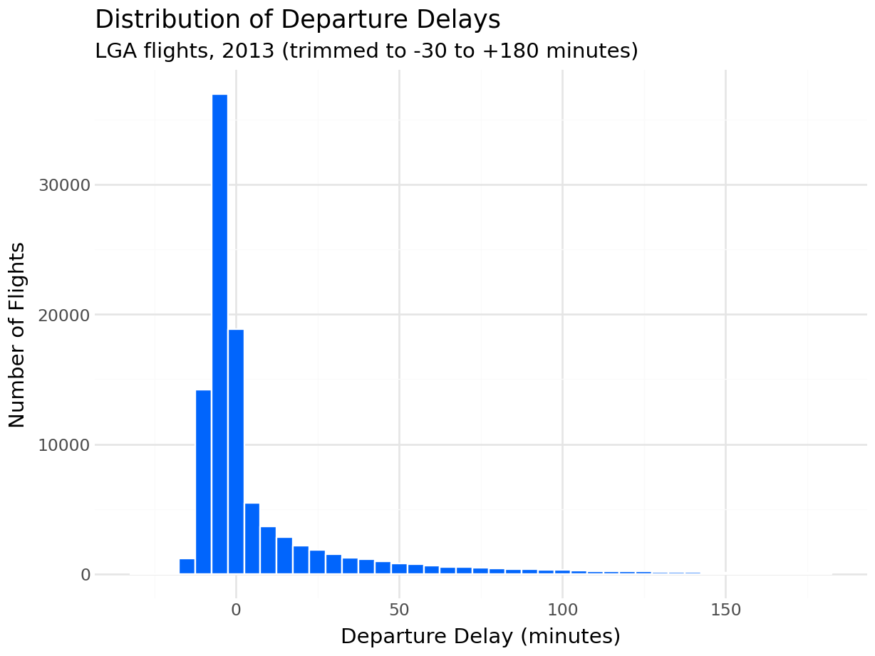
12.5.1 Distribution of Departure Delays
from plotnine import (
    ggplot, aes,
    geom_histogram, geom_point, geom_smooth, geom_col,
    coord_flip, labs, theme_minimal
)

delay_data = pl.read_database("""
    SELECT dep_delay
    FROM flights
    WHERE dep_delay IS NOT NULL
      AND dep_delay BETWEEN -30 AND 180
""", engine)

(
    ggplot(delay_data, aes(x="dep_delay"))
    + geom_histogram(binwidth=5, fill="#0165fc", color="white")
    + labs(
        title="Distribution of Departure Delays",
        subtitle="LGA flights, 2013 (trimmed to -30 to +180 minutes)",
        x="Departure Delay (minutes)",
        y="Number of Flights"
    )
    + theme_minimal()
)
import seaborn as sns
import matplotlib.pyplot as plt

delay_data_pd = pd.read_sql("""
    SELECT dep_delay
    FROM flights
    WHERE dep_delay IS NOT NULL
      AND dep_delay BETWEEN -30 AND 180
""", engine)

fig, ax = plt.subplots(figsize=(8, 4))
sns.histplot(data=delay_data_pd, x="dep_delay", binwidth=5, color="#0165fc", ax=ax)
ax.set_title("Distribution of Departure Delays")
ax.set_xlabel("Departure Delay (minutes)")
ax.set_ylabel("Number of Flights")
plt.tight_layout()
plt.show()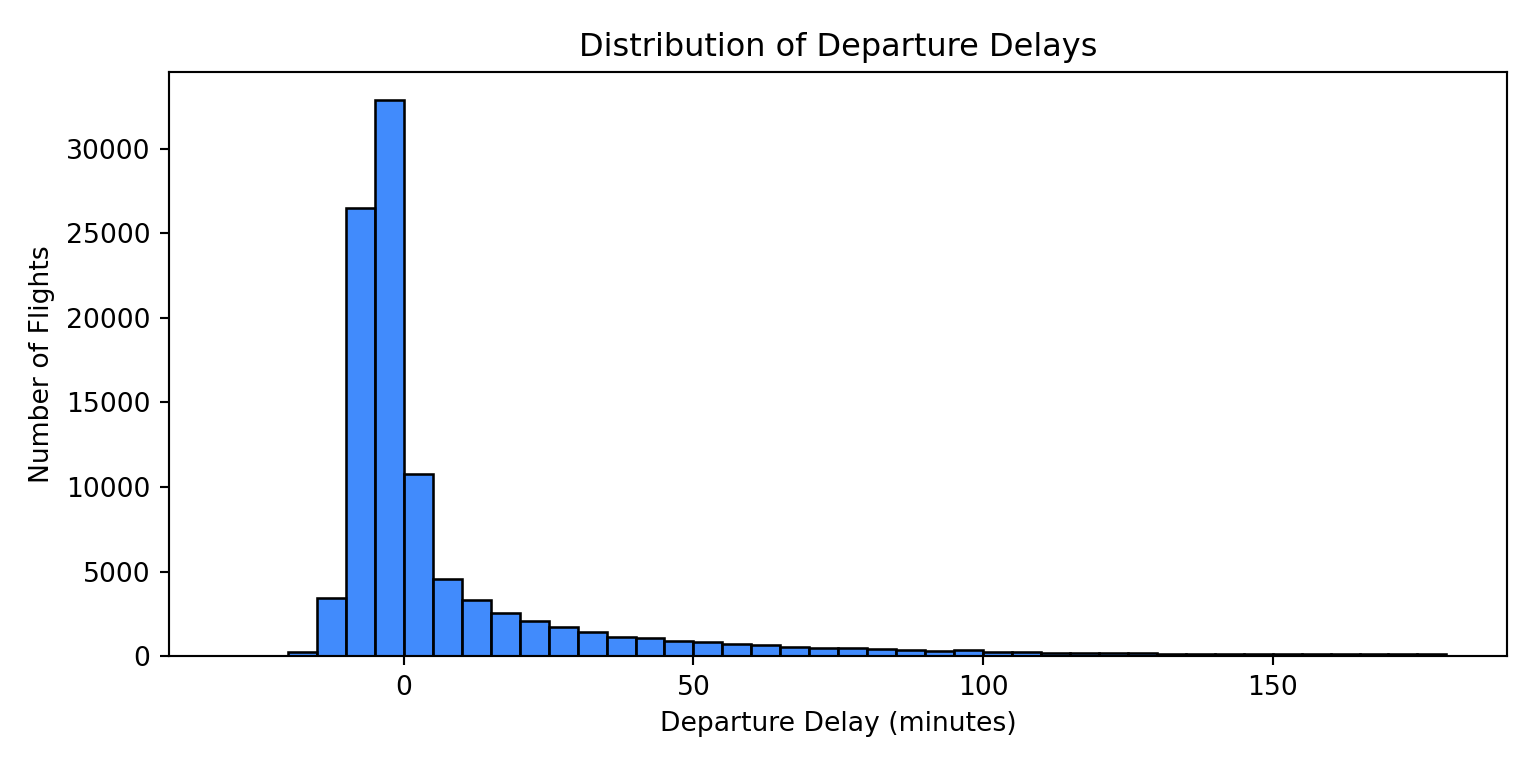
The right skew is unmistakable. The bulk of flights cluster just below zero, and a long tail of severe delays extends to the right.
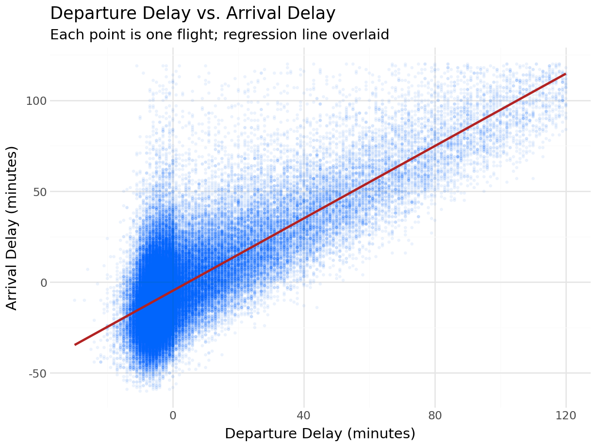
12.5.2 Departure Delay vs. Arrival Delay
delay_pairs = pl.read_database("""
    SELECT dep_delay, arr_delay
    FROM flights
    WHERE dep_delay IS NOT NULL
      AND arr_delay IS NOT NULL
      AND dep_delay BETWEEN -30 AND 120
      AND arr_delay BETWEEN -60 AND 120
""", engine)

(
    ggplot(delay_pairs, aes(x="dep_delay", y="arr_delay"))
    + geom_point(alpha=0.05, color="#0165fc", size=0.5)
    + geom_smooth(method="lm", color="firebrick", se=False)
    + labs(
        title="Departure Delay vs. Arrival Delay",
        subtitle="Each point is one flight; regression line overlaid",
        x="Departure Delay (minutes)",
        y="Arrival Delay (minutes)"
    )
    + theme_minimal()
)
delay_pairs_pd = pd.read_sql("""
    SELECT dep_delay, arr_delay
    FROM flights
    WHERE dep_delay IS NOT NULL
      AND arr_delay IS NOT NULL
      AND dep_delay BETWEEN -30 AND 120
      AND arr_delay BETWEEN -60 AND 120
""", engine)

fig, ax = plt.subplots(figsize=(6, 5))
ax.scatter(delay_pairs_pd["dep_delay"], delay_pairs_pd["arr_delay"],
           alpha=0.03, color="#0165fc", s=5)
sns.regplot(data=delay_pairs_pd, x="dep_delay", y="arr_delay",
            scatter=False, color="firebrick", ax=ax)
ax.set_title("Departure Delay vs. Arrival Delay")
ax.set_xlabel("Departure Delay (minutes)")
ax.set_ylabel("Arrival Delay (minutes)")
plt.tight_layout()
plt.show()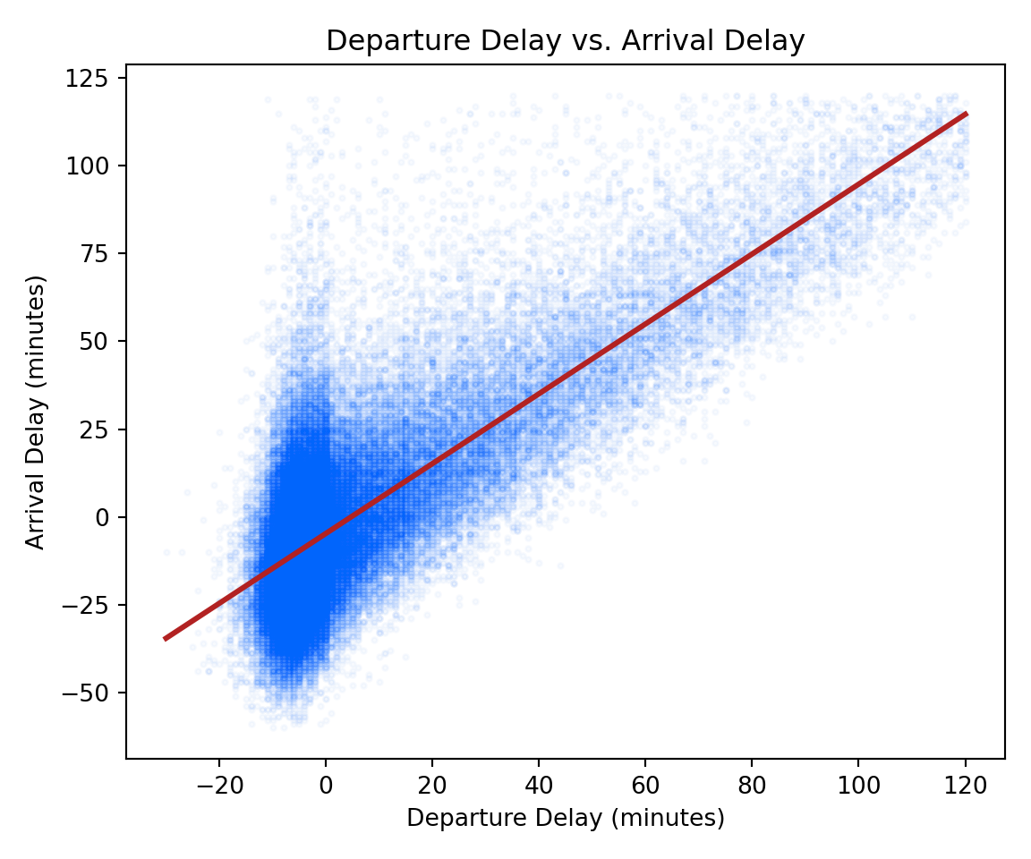
The regression line runs nearly through the origin with a slope close to 1: a one-minute departure delay corresponds to roughly one minute of arrival delay.
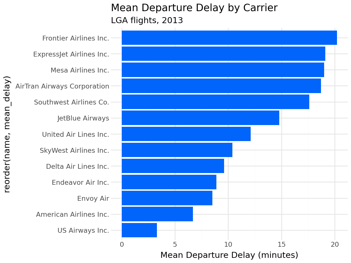
12.5.3 Mean Delay by Carrier
(
    ggplot(delays_by_carrier, aes(x="reorder(name, mean_delay)", y="mean_delay"))
    + geom_col(fill="#0165fc")
    + coord_flip()
    + labs(
        title="Mean Departure Delay by Carrier",
        subtitle="LGA flights, 2013",
        x=None,
        y="Mean Departure Delay (minutes)"
    )
    + theme_minimal()
)
delays_sorted = delays_by_carrier_pd.sort_values("mean_delay")

fig, ax = plt.subplots(figsize=(7, 5))
ax.barh(delays_sorted["name"], delays_sorted["mean_delay"], color="#0165fc")
ax.set_title("Mean Departure Delay by Carrier")
ax.set_xlabel("Mean Departure Delay (minutes)")
ax.set_ylabel(None)
plt.tight_layout()
plt.show()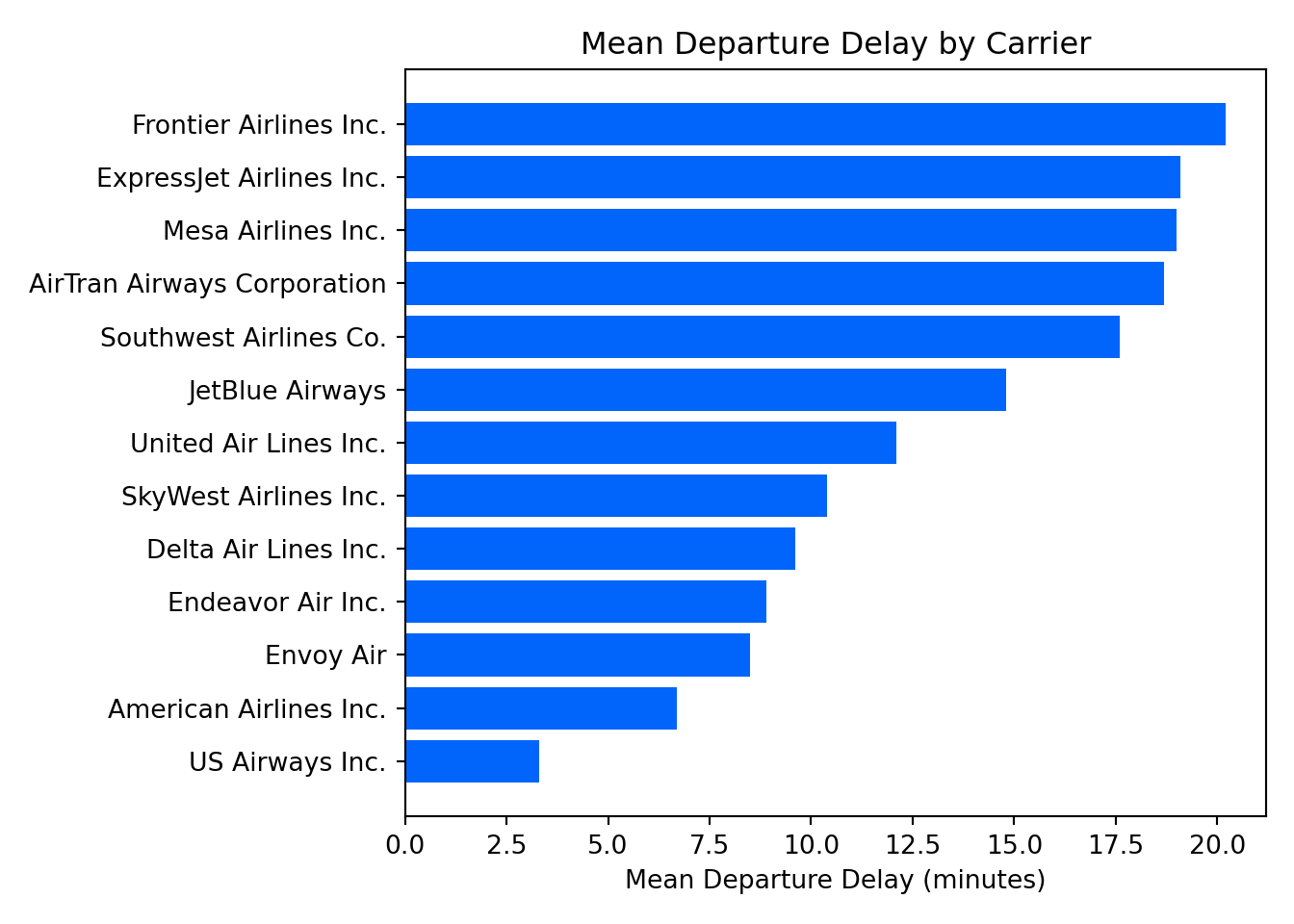
reorder(name, mean_delay) sorts the bars by delay value rather than alphabetically, making the ranking immediately visible — the same behavior as the reorder() call in ggplot2.
12.6 Parameterized Queries
Never interpolate Python values into a query string using f-strings or string concatenation. The same SQL injection risk that applies in R applies here. SQLAlchemy’s text() function supports named placeholders for safe value substitution:
# Do not do this
carrier_code = "AA"
pd.read_sql(f"SELECT * FROM flights WHERE carrier = '{carrier_code}'", engine)
The correct approach uses :param_name placeholders inside text(), with values passed as a separate dictionary:
from sqlalchemy import text

carrier_code = "AA"

with engine.connect() as conn:
    aa_flights = pd.read_sql(
        text("""
            SELECT flight, dep_delay, arr_delay, dest
            FROM flights
            WHERE carrier = :carrier
              AND dep_delay IS NOT NULL
            ORDER BY dep_delay DESC
        """),
        conn,
        params={"carrier": carrier_code}
    )

aa_flights.head()
flight dep_delay arr_delay dest
0 2019 803 802.0 STL
1 2437 660 648.0 MIA
2 731 613 598.0 DFW
3 753 533 499.0 DFW
4 731 504 493.0 DFWThe value of carrier_code is sent to the database separately from the query text. The driver handles quoting and escaping, so no injection is possible regardless of what the string contains. Multiple parameters follow the same pattern: add more :name placeholders and extend the dictionary.
Always use parameterized queries whenever a query incorporates a value that originates from outside your own code, including user input, configuration files, or data from another source. SQLAlchemy’s text() with named parameters is the right tool for raw SQL.
12.7 Exercises
12.7.1 Reflection
What is the role of SQLAlchemy in the Python database ecosystem? Why does using it as the connection layer allow you to switch between Polars and pandas without changing your connection code?
Explain what is wrong with building a query string using an f-string to insert a user-supplied value. What does a parameterized query do differently, and why does it prevent SQL injection?
Compare
plotnineandseabornas visualization libraries. In what way doesplotnine’s API differ fromseaborn’s, and what makesplotnineeasier to learn for someone who already knowsggplot2?
12.7.2 Coding
Connect to the
nycflightsdatabase and usepl.read_database()to retrieve the average temperature (temp) and average wind speed (wind_speed) from theweathertable, grouped by month. Print the result.Using
pl.read_database(), retrieve the number of flights per destination (dest). Then useplotnineto create a horizontal bar chart of the top 15 destinations by flight count.Write a parameterized query using SQLAlchemy’s
text()that accepts a destination airport code and returns the average departure delay for flights to that destination, grouped by carrier. Test it with at least two destination codes.Retrieve daily average departure delay from
flights(aggregate bymonthandday). Load the result into a Polars DataFrame, construct a date column frommonthandday, and plot the result as a line chart usingplotnine. Describe the seasonal pattern you observe.