In Development: This textbook is currently
undergoing development and should not be used as an authoritative
source of... well, ANYTHING.
6Joining Tables
6.1 Learning Objectives
By the end of this chapter, students will be able to:
Explain what a join is and why it is necessary when data is spread across multiple related tables.
Write an INNER JOIN to combine rows from two tables based on a matching key column.
Apply a LEFT JOIN to preserve all rows from the left table, including those with no match on the right.
Distinguish between INNER JOIN, LEFT JOIN, RIGHT JOIN, and FULL OUTER JOIN and predict the row count each produces for a given pair of tables.
Use table aliases to write more concise and readable join queries.
Write a query that joins three or more tables in a single statement.
Apply a self-join to compare or relate rows within the same table.
UseCROSS JOIN to produce a Cartesian product and identify a practical scenario where this is the intended behavior.
Diagnose unexpected duplicate rows caused by one-to-many join relationships and correct the query.
Select the appropriate join type for a given analytical question.
Every query you have written so far has drawn from a single table. That is useful, but it is not the whole story. Real databases almost always store related information across multiple tables, and one of SQL’s most powerful capabilities is the ability to combine those tables into a single result. That operation is called a join.
This chapter explains why data is structured across multiple tables in the first place, introduces the key concepts of primary keys, foreign keys, and cardinality, and then walks through every major join type with diagrams and examples. By the end, you will be able to assemble information from several related tables into exactly the view you need.
6.2 Keys and Relationships
To understand joins, you first need to understand how tables are related to each other. Relational databases are built around the idea that data should be stored once and referenced many times, rather than repeated in every table that needs it. The mechanism that makes this possible is the relationship between tables, expressed through keys.
6.2.1 Primary Keys
A primary key is a column, or combination of columns, whose values uniquely identify each row in a table. No two rows in a table can share the same primary key value, and the primary key column cannot be NULL.
Primary keys come in two common forms:
Natural keys use a value that already exists in the data and is inherently unique, such as a country’s three-letter ISO code or a flight number.
Surrogate keys are artificial values added solely to serve as identifiers, typically auto-incrementing integers (1, 2, 3, …) with no meaning outside the database.
Natural keys are intuitive but can cause problems if the “unique” real-world value turns out to change or repeat. Surrogate keys are more stable, which is why they appear so frequently in production databases.
When no single column is sufficient to uniquely identify every row, two or more columns together can serve as the primary key. This is called a composite primary key. The indicators table in this chapter is a good example: neither country_id nor year is unique on its own, but the combination of the two identifies exactly one row, the measurements recorded for that country in that year.
6.2.2 Foreign Keys
A foreign key is a column in one table that holds values matching the primary key of another table. It is the bridge between two tables and the foundation of every join.
For example, the indicators table has a column called country_id, and the countries table has id as its primary key. The column indicators.country_id is a foreign key pointing to countries.id. Every value in indicators.country_id should correspond to a row that actually exists in countries. This guarantee is called referential integrity, and the database can enforce it automatically once the foreign key relationship is declared.
The table that holds the foreign key is called the child table. The table being referenced is the parent table. In this example, indicators is the child and countries is the parent.
6.2.3 Cardinality
Cardinality describes how many rows in one table can relate to how many rows in another. There are three fundamental patterns.
One-to-one. Each row in Table A corresponds to at most one row in Table B, and vice versa. This pattern is relatively rare. It sometimes appears when a large table is split in two for organizational or access-control reasons.
One-to-many. Each row in Table A can relate to many rows in Table B, but each row in Table B relates to exactly one row in Table A. This is the most common cardinality in relational databases. One country can have many rows in indicators, one for each year that data was recorded. Each indicator row, in turn, belongs to exactly one country.
Many-to-many. Each row in Table A can relate to many rows in Table B, and each row in Table B can relate to many rows in Table A. A student can be enrolled in many courses, and the same course can have many students. This relationship cannot be expressed with just two tables. It requires a third table, often called a junction table or bridge table, whose rows each pair one row from Table A with one row from Table B.
Understanding cardinality before writing a join is important because it tells you how many result rows to expect. Joining a parent table to a child in a one-to-many relationship will produce more rows than the parent table alone, one result row for each matching child. Forgetting this is a common source of unintentionally duplicated rows.
This chapter introduces primary keys, foreign keys, and cardinality as the practical foundation for writing joins. The database design section later in this book covers all three in greater depth, including how to declare and enforce them in SQL using CREATE TABLE statements and column constraints, and how normalization principles guide decisions about table structure.
6.3 The worldbank Database
The examples in this chapter use the worldbank database, which contains three tables drawn from World Bank development data.
Table
Primary Key
Description
countries
id
One row per country or territory (299 rows)
indicators
(country_id, year)
One row per country-year with multiple measurement columns (16,704 rows)
series
id
Metadata describing each measurement type (9 rows)
The only enforced foreign key relationship is:
indicators.country_id references countries.id
The countries table includes both individual countries and regional aggregates such as “Africa” and “High income”. These 38 aggregate entries appear in countries but have no corresponding rows in indicators, which records data only for individual countries. That natural gap is what makes the left join and anti-join examples in this chapter meaningful.
The indicators table stores measurements as columns rather than rows. Each row captures one country in one year, and columns like gdp_per_capita_usd, population, pct_forest_area, and land_area_km2 hold the values for that combination. Data spans from 1960 through 2023.
The series table describes what each measurement type means, including indicator codes, names, and source descriptions. It is not linked to indicators by a foreign key, but it is a useful reference when you want to understand what a particular column represents.
6.4 JOIN Syntax
Before looking at specific join types, it helps to see the general shape of a join query.
SELECT c.short_name, i.gdp_per_capita_usdFROM countries AS cJOIN indicators AS i ON c.id= i.country_id;
A few things to note.
Table aliases. The AS c and AS i after each table name assign short aliases. These are optional but almost universally used when joining tables, because they make it possible to refer to columns unambiguously without typing the full table name each time.
Column qualification. When two tables share a column name, you must prefix the column name with the table alias to tell the database which one you mean. Writing c.id instead of just id prevents ambiguity. Even when column names do not overlap, qualifying them explicitly is good practice in join queries because it makes it immediately clear where each column originates.
The ON clause. This is where you specify the condition that links the two tables. Almost always this is an equality between a foreign key in one table and the primary key in another, though more complex conditions are possible.
PostgreSQL also supports a USING clause as a shorthand when both tables share an identically named join column:
FROM table_aJOIN table_b USING (shared_column_name)
USING is concise but requires the join columns to carry the same name in both tables. Because countries uses id while indicators uses country_id, this particular join must use ON. Throughout this book, all examples use ON for clarity and consistency.
6.5 Reading the Diagrams
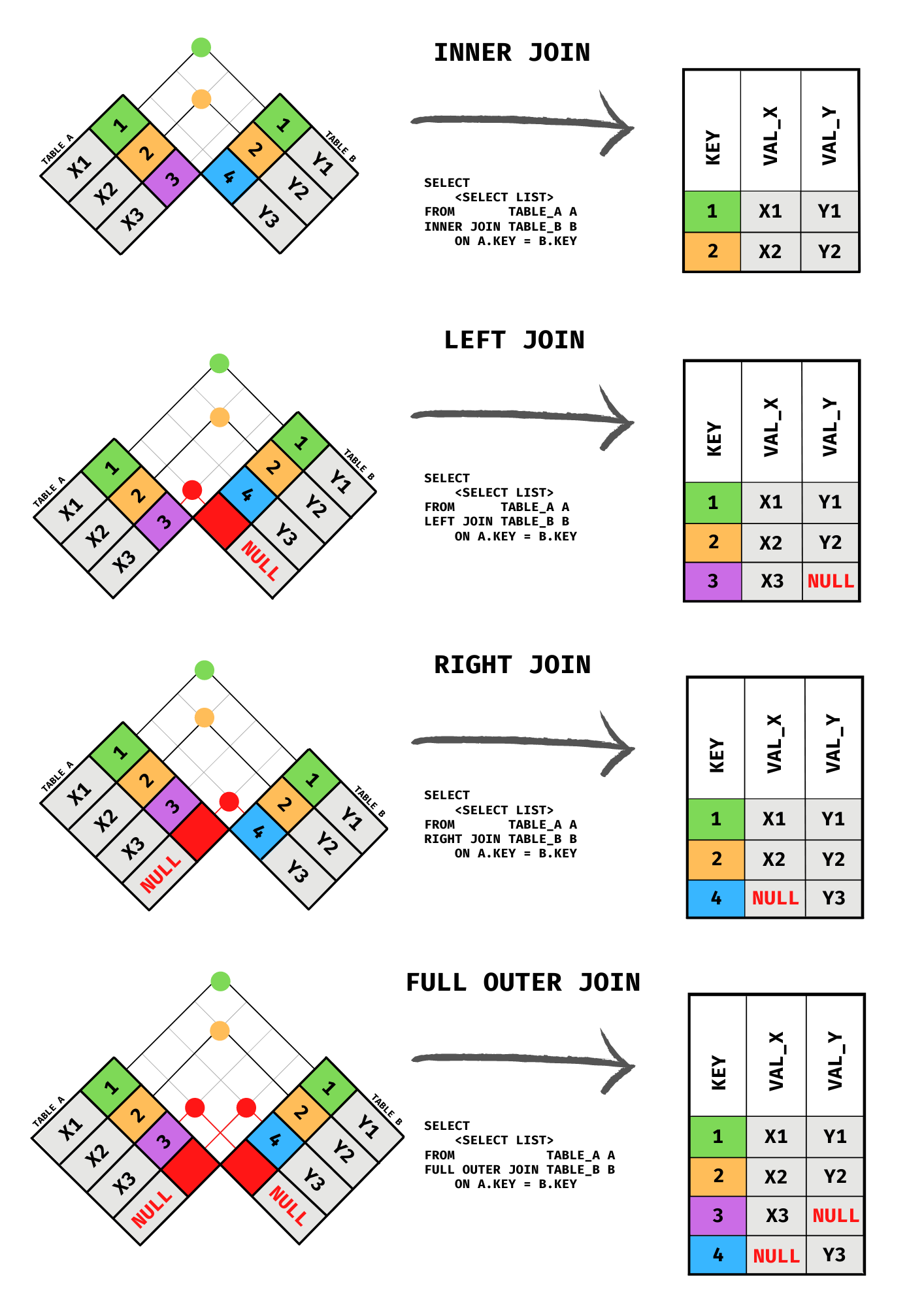
The diagrams in this chapter use the checkered flag method to illustrate joins. Each diagram shows two tables arranged as rotated grids facing each other. Color-coded cells identify which rows from each table contribute to the result, and a result table on the right shows the output.
This approach is deliberately different from the Venn diagrams you may have seen elsewhere. Venn diagrams are not entirely wrong — Codd’s relational model defines a relation as an unordered set of tuples, so the set-based intuition has a legitimate foundation. The problem is more subtle. A Venn diagram implies that the “intersection” consists of rows that are identical members of both tables, the way the number 3 might belong to both Set A and Set B. A SQL join does not work that way. The two tables being joined typically contain different things entirely, and the join matches rows across them based on a condition you specify, usually a foreign key relationship. There is no literal overlap of identical elements. Venn diagrams also fail to convey cardinality: when one country joins to many yearly measurements, the result has one row per measurement, but the overlapping-circles picture gives no indication of that. The checkered flag diagrams make the row-matching process explicit, showing which rows from each table appear in the result and how NULLs fill in for unmatched rows in outer joins.
INNER JOIN, LEFT JOIN, RIGHT JOIN, and FULL OUTER JOIN illustrated with the checkered flag method.
6.6 INNER JOIN
An INNER JOIN returns only the rows where the join condition is satisfied in both tables. Rows that have no match on the other side are excluded from the result entirely.
This is the default join type. Writing JOIN without a qualifier is equivalent to writing INNER JOIN.
SELECT c.short_name, c.region, i.gdp_per_capita_usd, i.populationFROM countries AS cINNERJOIN indicators AS i ON c.id= i.country_idWHERE i.year=2022ORDERBY i.gdp_per_capita_usd DESCNULLSLASTLIMIT10;
10 records
short_name
region
gdp_per_capita_usd
population
Monaco
Europe & Central Asia
226052.00
5
Liechtenstein
Europe & Central Asia
186400.23
39493
Luxembourg
Europe & Central Asia
125006.02
653103
Bermuda
North America
120897.31
64749
Norway
Europe & Central Asia
108798.45
5457127
Ireland
Europe & Central Asia
106194.76
5165700
Switzerland
Europe & Central Asia
93245.80
8777088
Cayman Islands
Latin America & Caribbean
92202.15
71591
Qatar
Middle East & North Africa
88701.46
2657333
Singapore
East Asia & Pacific
88428.70
5637022
This query pairs each country with its 2022 measurements. Because the join is inner, any country without a matching row in indicators is excluded from the result entirely. Notice that no entries from the Aggregates region appear: the 38 regional aggregates in countries have no rows in indicators, so the inner join drops them without any warning. The next section shows how a left join makes those gaps visible.
When a column name exists in only one of the joined tables, you can reference it without a qualifier and PostgreSQL will resolve it unambiguously. However, any column name that appears in more than one table must be qualified with the table alias, or the query will fail with an “ambiguous column” error. When in doubt, qualify every column.
6.7 LEFT JOIN
A LEFT JOIN (also written LEFT OUTER JOIN) returns all rows from the left table and the matching rows from the right table. Where no match exists in the right table, the right-side columns are filled with NULL.
The “left” table is the one named in the FROM clause. The “right” table is the one named in the JOIN clause.
SELECT c.short_name, c.region, i.year, i.populationFROM countries AS cLEFTJOIN indicators AS i ON c.id= i.country_idORDERBY c.short_name, i.yearLIMIT15;
15 records
short_name
region
year
population
Afghanistan
South Asia
1960
9035043
Afghanistan
South Asia
1961
9214083
Afghanistan
South Asia
1962
9404406
Afghanistan
South Asia
1963
9604487
Afghanistan
South Asia
1964
9814318
Afghanistan
South Asia
1965
10036008
Afghanistan
South Asia
1966
10266395
Afghanistan
South Asia
1967
10505959
Afghanistan
South Asia
1968
10756922
Afghanistan
South Asia
1969
11017409
Afghanistan
South Asia
1970
11290128
Afghanistan
South Asia
1971
11567667
Afghanistan
South Asia
1972
11853696
Afghanistan
South Asia
1973
12157999
Afghanistan
South Asia
1974
12469127
The first rows in this result belong to regional aggregates such as “Africa” and “Africa Eastern and Southern”. They appear with NULL in both year and population because they have no rows in indicators. Further down, individual countries appear once per year of recorded data. The left join preserves every row from countries, whether or not a match exists on the right side.
Left joins are extremely common in analytical queries because they let you start with a complete reference list (all countries) and attach available data without discarding entries that happen to have gaps.
6.7.1 ON vs. WHERE: When Filter Placement Matters
Every join query can have two places where you restrict rows: inside the ON clause and inside the WHERE clause. Understanding the difference is one of the most important skills in SQL, because the two clauses run at different stages of query execution and produce different results with outer joins.
The ON clause runs during the join itself. It controls which rows from the right table are even considered as candidates for matching against each left-table row. Rows that fail the ON condition are not matched, but in an outer join, the left-table row still appears in the result with NULLs on the right side.
The WHERE clause runs after the join is complete. It filters the already-assembled result set. Any row that does not satisfy WHERE is discarded, NULLs and all.
With INNER JOIN, the placement makes no difference. Because an inner join already discards rows with no match, there are no NULL-padded rows for a WHERE filter to remove. These two queries return identical results:
SELECT c.short_name, i.year, i.gdp_per_capita_usdFROM countries AS cINNERJOIN indicators AS i ON c.id= i.country_idWHERE i.year=2022ORDERBY c.short_nameLIMIT5;
5 records
short_name
year
gdp_per_capita_usd
Afghanistan
2022
357.26
Africa Eastern and Southern
2022
1628.02
Africa Western and Central
2022
1777.24
Albania
2022
6846.43
Algeria
2022
4961.55
SELECT c.short_name, i.year, i.gdp_per_capita_usdFROM countries AS cINNERJOIN indicators AS iON c.id= i.country_id AND i.year=2022ORDERBY c.short_nameLIMIT5;
5 records
short_name
year
gdp_per_capita_usd
Afghanistan
2022
357.26
Africa Eastern and Southern
2022
1628.02
Africa Western and Central
2022
1777.24
Albania
2022
6846.43
Algeria
2022
4961.55
With LEFT JOIN (and other outer joins), the placement is critical. Suppose you want every country alongside its 2022 GDP figure, with NULL for countries that have no 2022 data. This query does not accomplish that goal:
SELECT c.short_name, c.region, i.year, i.gdp_per_capita_usdFROM countries AS cLEFTJOIN indicators AS i ON c.id= i.country_idWHERE i.year=2022ORDERBY c.short_nameLIMIT10;
10 records
short_name
region
year
gdp_per_capita_usd
Afghanistan
South Asia
2022
357.26
Africa Eastern and Southern
Aggregates
2022
1628.02
Africa Western and Central
Aggregates
2022
1777.24
Albania
Europe & Central Asia
2022
6846.43
Algeria
Middle East & North Africa
2022
4961.55
American Samoa
East Asia & Pacific
2022
18017.46
Andorra
Europe & Central Asia
2022
42414.06
Angola
Sub-Saharan Africa
2022
2929.69
Antigua and Barbuda
Latin America & Caribbean
2022
20117.77
Arab World
Aggregates
2022
7658.41
The left join runs first and correctly produces 16,742 rows: 16,704 matched rows plus 38 NULL-padded rows for the regional aggregates. Then WHERE i.year = 2022 runs on that result and discards every row where i.year is NULL, which are exactly the 38 unmatched rows. The left join’s promise of “all left rows” is silently undone, and the result is identical to an inner join.
Moving the condition into the ON clause fixes it:
SELECT c.short_name, c.region, i.year, i.gdp_per_capita_usdFROM countries AS cLEFTJOIN indicators AS iON c.id= i.country_idAND i.year=2022ORDERBY c.short_nameLIMIT15;
15 records
short_name
region
year
gdp_per_capita_usd
Afghanistan
South Asia
2022
357.26
Africa
Aggregates
NULL
NULL
Africa Eastern and Southern
Aggregates
2022
1628.02
Africa Western and Central
Aggregates
2022
1777.24
Albania
Europe & Central Asia
2022
6846.43
Algeria
Middle East & North Africa
2022
4961.55
American Samoa
East Asia & Pacific
2022
18017.46
Andorra
Europe & Central Asia
2022
42414.06
Angola
Sub-Saharan Africa
2022
2929.69
Antigua and Barbuda
Latin America & Caribbean
2022
20117.77
Arab World
Aggregates
2022
7658.41
Argentina
Latin America & Caribbean
2022
13935.68
Armenia
Europe & Central Asia
2022
6571.97
Aruba
Latin America & Caribbean
2022
30559.53
Australia
East Asia & Pacific
2022
64997.01
Now the database evaluates i.year = 2022 during the join. For each country row, it looks for a matching indicator row where both country_id matches and year equals 2022. If no such row exists, the country still appears in the result, with NULLs on the right side. All 299 rows from countries come through.
The practical rule: conditions that restrict which right-table rows qualify as a match belong in ON; conditions that should discard rows from the final result regardless of match status belong in WHERE. For inner joins the distinction is academic. For any outer join it is not.
6.7.2 RIGHT JOIN
A RIGHT JOIN is the mirror image of a LEFT JOIN. It returns all rows from the right table and the matching rows from the left, filling unmatched left-side columns with NULL.
SELECT c.short_name, i.year, i.populationFROM countries AS cRIGHTJOIN indicators AS i ON c.id= i.country_idORDERBY c.short_name, i.yearLIMIT10;
10 records
short_name
year
population
Afghanistan
1960
9035043
Afghanistan
1961
9214083
Afghanistan
1962
9404406
Afghanistan
1963
9604487
Afghanistan
1964
9814318
Afghanistan
1965
10036008
Afghanistan
1966
10266395
Afghanistan
1967
10505959
Afghanistan
1968
10756922
Afghanistan
1969
11017409
This returns every row from indicators, with the country name attached from the left table. Because indicators.country_id is enforced as a foreign key, every indicator row already has a valid matching country, so no NULLs appear on the left side here.
In practice, RIGHT JOIN is used infrequently. Any right join can be rewritten as a left join by swapping the order of the tables, which most developers find more readable. The queries below produce identical results:
FROM countries AS cRIGHTJOIN indicators AS i ON c.id= i.country_idFROM indicators AS iLEFTJOIN countries AS c ON c.id= i.country_id
6.8 FULL OUTER JOIN
A FULL OUTER JOIN returns all rows from both tables. Rows that have a match are joined together. Rows from the left table with no right-side match appear with NULLs on the right. Rows from the right table with no left-side match appear with NULLs on the left.
SELECT c.short_name, c.region, i.gdp_per_capita_usdFROM countries AS cFULLOUTERJOIN indicators AS iON c.id= i.country_idAND i.year=2022ORDERBY c.short_nameLIMIT20;
20 records
short_name
region
gdp_per_capita_usd
Afghanistan
South Asia
357.26
Africa
Aggregates
NULL
Africa Eastern and Southern
Aggregates
1628.02
Africa Western and Central
Aggregates
1777.24
Albania
Europe & Central Asia
6846.43
Algeria
Middle East & North Africa
4961.55
American Samoa
East Asia & Pacific
18017.46
Andorra
Europe & Central Asia
42414.06
Angola
Sub-Saharan Africa
2929.69
Antigua and Barbuda
Latin America & Caribbean
20117.77
Arab World
Aggregates
7658.41
Argentina
Latin America & Caribbean
13935.68
Armenia
Europe & Central Asia
6571.97
Aruba
Latin America & Caribbean
30559.53
Australia
East Asia & Pacific
64997.01
Austria
Europe & Central Asia
52176.66
Azerbaijan
Europe & Central Asia
7770.59
Bahamas, The
Latin America & Caribbean
33044.39
Bahrain
Middle East & North Africa
30616.26
Bangladesh
South Asia
2716.49
Because indicators.country_id is enforced as a foreign key, every indicator row already has a matching country. The only unmatched rows come from the left side: the 38 aggregates in countries with no indicator data. The result is therefore the same as a left join with the year in the ON clause. Full outer joins show their full value when comparing two datasets that are not constrained to reference each other, such as two independent snapshots of the same data where either side could contain records the other does not.
6.9 CROSS JOIN
A CROSS JOIN produces the Cartesian product of two tables: every row from the left table is paired with every row from the right table. If the left table has M rows and the right table has N rows, the result has M × N rows. No join condition is specified.
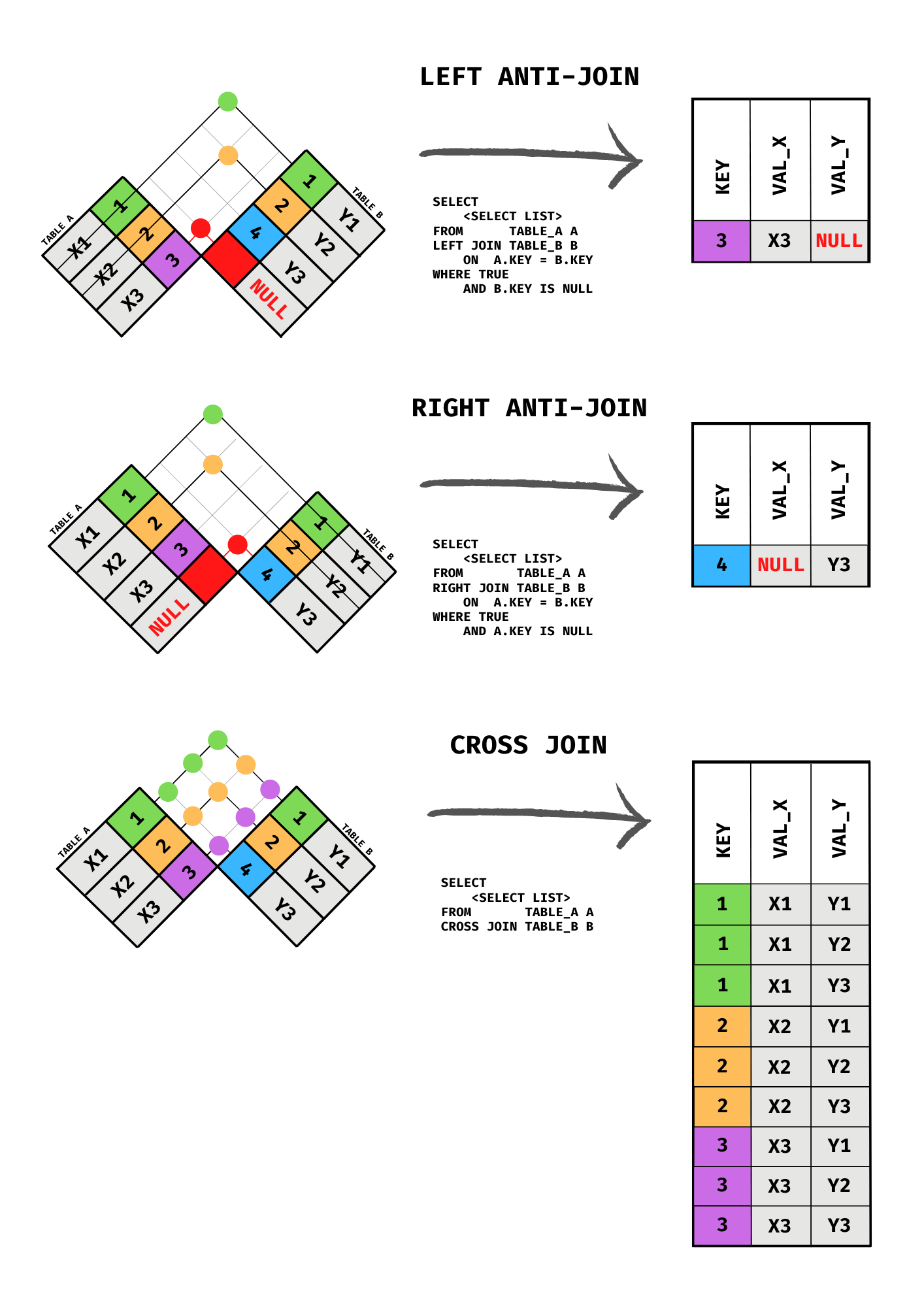
LEFT ANTI-JOIN, RIGHT ANTI-JOIN, and CROSS JOIN illustrated with the checkered flag method.
The series table, with its 9 rows describing each measurement type, pairs naturally with countries in a cross join. The result is a complete grid of every possible country-indicator combination.
SELECT c.short_name, s.indicator_nameFROM countries AS cCROSSJOIN series AS sORDERBY c.short_name, s.indicator_nameLIMIT15;
15 records
short_name
indicator_name
Afghanistan
Agricultural land (% of land area)
Afghanistan
Arable land (% of land area)
Afghanistan
Forest area (% of land area)
Afghanistan
GDP (current US\() |
|Afghanistan |GDP per capita (current US\))
Afghanistan
Land area (sq. km)
Afghanistan
Population, total
Afghanistan
Rural land area (sq. km)
Afghanistan
Urban land area (sq. km)
Africa
Agricultural land (% of land area)
Africa
Arable land (% of land area)
Africa
Forest area (% of land area)
Africa
GDP (current US\() |
|Africa |GDP per capita (current US\))
Africa
Land area (sq. km)
With 299 countries and 9 indicator types, this produces 2,691 rows. Cross joins grow very quickly.
Accidental cross joins are one of the most common sources of runaway queries in SQL. They happen when a join condition is missing or typo’d, causing the database to pair every row with every other row. Always verify that a JOIN clause has an ON condition unless you genuinely intend a cross join.
Intentional cross joins do have legitimate uses. Generating all possible combinations of two dimensions, such as every country paired with every indicator type to build a complete reporting grid with no gaps, is a situation where a cross join is exactly the right tool.
6.10 Anti-Joins
An anti-join returns rows from one table that have no matching row in the other table. It is the complement of an inner join.
Anti-joins do not have a dedicated keyword in SQL. They are expressed using one of two patterns.
6.10.1 Using LEFT JOIN and IS NULL
The most common pattern extends a left join with a WHERE clause that keeps only the rows where the right side produced a NULL, meaning no match was found.
SELECT c.short_name, c.regionFROM countries AS cLEFTJOIN indicators AS i ON c.id= i.country_idWHERE i.country_id ISNULL;
Displaying records 1 - 25
short_name
region
Africa
Aggregates
East Asia & Pacific (IBRD-only countries)
Aggregates
Europe & Central Asia (IBRD-only countries)
Aggregates
IBRD countries classified as high income
Aggregates
Latin America & the Caribbean (IBRD-only countries)
Aggregates
Middle East & North Africa (IBRD-only countries)
Aggregates
Sub-Saharan Africa (IBRD-only countries)
Aggregates
Sub-Saharan Africa (IFC classification)
Aggregates
East Asia and the Pacific (IFC classification)
Aggregates
Europe and Central Asia (IFC classification)
Aggregates
Latin America and the Caribbean (IFC classification)
Aggregates
Middle East and North Africa (IFC classification)
Aggregates
South Asia (IFC classification)
Aggregates
East Asia & Pacific (IDA-eligible countries)
Aggregates
Europe & Central Asia (IDA-eligible countries)
Aggregates
IDA countries classified as Fragile Situations
Aggregates
Latin America & the Caribbean (IDA-eligible countries)
Aggregates
Middle East & North Africa (IDA-eligible countries)
Aggregates
IDA countries not classified as Fragile Situations
Aggregates
IDA countries in Sub-Saharan Africa not classified as fragile situations
Aggregates
South Asia (IDA-eligible countries)
Aggregates
IDA countries in Sub-Saharan Africa classified as fragile situations
Aggregates
Sub-Saharan Africa (IDA-eligible countries)
Aggregates
IDA countries classified as fragile situations, excluding Sub-Saharan Africa
Aggregates
High income
Aggregates
This returns every entry in countries that has no rows in indicators. The left join brings in all countries; the WHERE clause discards the ones that did match, leaving only those that did not. The result is the 38 regional aggregate entries.
Filter on the join key column from the right table, not a data column. The join key is guaranteed to be NULL only when no match was found. A data column could be NULL for other reasons, which would produce false positives.
6.10.2 Using NOT EXISTS
The second pattern uses NOT EXISTS with a correlated subquery. This is the approach mentioned in the WHERE clause chapter as the preferred alternative to NOT IN when NULL values may be present.
SELECT c.short_name, c.regionFROM countries AS cWHERENOTEXISTS (SELECT1FROM indicators AS iWHERE i.country_id = c.id);
Displaying records 1 - 25
short_name
region
Africa
Aggregates
East Asia & Pacific (IBRD-only countries)
Aggregates
Europe & Central Asia (IBRD-only countries)
Aggregates
IBRD countries classified as high income
Aggregates
Latin America & the Caribbean (IBRD-only countries)
Aggregates
Middle East & North Africa (IBRD-only countries)
Aggregates
Sub-Saharan Africa (IBRD-only countries)
Aggregates
Sub-Saharan Africa (IFC classification)
Aggregates
East Asia and the Pacific (IFC classification)
Aggregates
Europe and Central Asia (IFC classification)
Aggregates
Latin America and the Caribbean (IFC classification)
Aggregates
Middle East and North Africa (IFC classification)
Aggregates
South Asia (IFC classification)
Aggregates
East Asia & Pacific (IDA-eligible countries)
Aggregates
Europe & Central Asia (IDA-eligible countries)
Aggregates
IDA countries classified as Fragile Situations
Aggregates
Latin America & the Caribbean (IDA-eligible countries)
Aggregates
Middle East & North Africa (IDA-eligible countries)
Aggregates
IDA countries not classified as Fragile Situations
Aggregates
IDA countries in Sub-Saharan Africa not classified as fragile situations
Aggregates
South Asia (IDA-eligible countries)
Aggregates
IDA countries in Sub-Saharan Africa classified as fragile situations
Aggregates
Sub-Saharan Africa (IDA-eligible countries)
Aggregates
IDA countries classified as fragile situations, excluding Sub-Saharan Africa
Aggregates
High income
Aggregates
The subquery runs once for each row in countries, checking whether any matching row exists in indicators. If none is found, NOT EXISTS returns TRUE and the country is included in the result.
Both patterns produce the same rows. The LEFT JOIN / IS NULL form is often more familiar to beginners. The NOT EXISTS form can be faster on large tables and handles NULL values in the join key more predictably, which is why many experienced SQL writers prefer it.
6.11 Joining More Than Two Tables
Nothing limits a query to two tables. You can chain as many joins as the data requires, adding one table at a time. One particularly useful pattern is joining the same table twice under different aliases to compare values across two points in time. Here, the indicators table is joined twice to place 2000 and 2022 GDP figures side by side.
SELECT c.short_name, c.region, i2000.gdp_per_capita_usd AS gdp_2000, i2022.gdp_per_capita_usd AS gdp_2022FROM countries AS cINNERJOIN indicators AS i2000ON c.id= i2000.country_id AND i2000.year=2000INNERJOIN indicators AS i2022ON c.id= i2022.country_id AND i2022.year=2022WHERE c.region !='Aggregates'ORDERBY c.short_nameLIMIT10;
10 records
short_name
region
gdp_2000
gdp_2022
Afghanistan
South Asia
174.93
357.26
Albania
Europe & Central Asia
1126.68
6846.43
Algeria
Middle East & North Africa
1772.93
4961.55
American Samoa
East Asia & Pacific
NULL
18017.46
Andorra
Europe & Central Asia
21810.25
42414.06
Angola
Sub-Saharan Africa
563.73
2929.69
Antigua and Barbuda
Latin America & Caribbean
12021.46
20117.77
Argentina
Latin America & Caribbean
7637.01
13935.68
Armenia
Europe & Central Asia
593.45
6571.97
Aruba
Latin America & Caribbean
20681.02
30559.53
Each instance of the indicators table gets its own alias (i2000 and i2022) so the query can reference columns from each independently. The year condition is placed inside the ON clause for each join so it participates in the matching logic rather than filtering the result after the fact.
Because both joins are inner, only countries with data for both 2000 and 2022 appear. Countries that were not yet sovereign in 2000, such as South Sudan (independence: 2011), are silently excluded. If you need to preserve countries that have data for only one of the two years, replace the inner joins with left joins.
A few practical notes on multi-table joins:
Start from the table that drives the query. If you want one row per country, start from countries. If you want one row per year-measurement, start from indicators. The starting table sets the row grain of the result.
Each join adds columns, not necessarily rows. A join to a parent table in a many-to-one relationship (indicators to countries) does not change the number of rows. A join to a child table in a one-to-many relationship (countries to indicators) multiplies rows. Understanding this keeps the result size predictable.
Order joins for readability. SQL does not require joins in any particular sequence, but organizing them so that each new table connects to something already in the query makes the logic easier to follow.
6.12 Implicit vs. Explicit Join Syntax
SQL has two ways to join tables. The style used throughout this book is the explicit syntax, introduced in the ANSI SQL-92 standard, where the join type and condition are stated directly:
FROM countries AS cINNERJOIN indicators AS i ON c.id= i.country_id
Before SQL-92, the only option was the implicit syntax: tables are comma-separated in the FROM clause and the join condition appears in WHERE alongside any other filters. The AS keyword for aliases is also commonly omitted in this style.
The result is identical to the explicit INNER JOIN from earlier in this chapter. Implicit joins still execute in every major SQL database and appear frequently in legacy code, older textbooks, and online examples, so you will encounter them.
There are three reasons to use explicit syntax for any new work.
Join conditions and filter conditions are visually indistinguishable. In the implicit style, c.id = i.country_id (a join condition) and i.year = 2022 (a data filter) both sit in WHERE with no structural difference between them. With explicit syntax, join conditions live in ON and filters live in WHERE, so the purpose of each clause is immediately clear.
A missing join condition silently produces a cross join. If the condition linking the two tables is accidentally left out in the implicit style, the database returns the Cartesian product without any warning or error:
SELECTCOUNT(*)FROM countries, indicators;
1 records
count
4994496
With explicit syntax, omitting the ON clause is a syntax error that fails immediately rather than quietly returning millions of rows.
Outer joins require explicit syntax. There is no comma-table equivalent of LEFT JOIN or FULL OUTER JOIN. Some databases offered proprietary workarounds (Oracle’s (+) operator, for example), but they were not portable and are now deprecated. Any query that needs to preserve unmatched rows must use explicit syntax.
6.13 Exercises
6.13.1 Reflection
Explain the difference between a primary key and a foreign key. Why does a database need both?
A data analyst runs an inner join between countries (299 rows) and indicators without filtering by year and gets back over 16,000 rows. They suspect something went wrong. Is this necessarily a problem? Explain what produces a result with many more rows than the starting table.
What is the difference between putting a filter condition in the ON clause of a left join versus putting it in the WHERE clause? When does the placement matter?
Describe two different SQL patterns that produce an anti-join. In what circumstances might you prefer one over the other?
You find the following query in a legacy codebase: SELECT c.short_name, i.population FROM countries c, indicators i WHERE c.id = i.country_id AND i.year = 2010. Rewrite it using explicit join syntax. Does the rewrite change the result?
6.13.2 Coding
Write a query that returns the short_name, region, and 2022 gdp_per_capita_usd for every country that has 2022 data in the indicators table. Exclude regional aggregates (where region = 'Aggregates'). Sort by gdp_per_capita_usd descending, with NULLs last. Limit to 20 rows.
Write a query that returns every country along with its 2010 gdp_per_capita_usd. Countries that have no 2010 data should still appear in the result, with NULL in the GDP column. Sort by short_name.
Write a query that returns the short_name and region of every entry in countries that has no rows at all in the indicators table. Use the LEFT JOIN / IS NULL pattern.
Rewrite the query from exercise 7 using NOT EXISTS instead of LEFT JOIN / IS NULL. Confirm that both queries return the same set of entries.
Write a query that returns each country’s short_name, region, and GDP per capita for both 1990 and 2022 side by side. Name the GDP columns gdp_1990 and gdp_2022. Include only countries that have data for both years, and exclude regional aggregates. Sort by short_name.