In Development: This textbook is currently undergoing development and should not be used as an authoritative source of... well, ANYTHING.

11  Connecting R to a Database

11.1 Learning Objectives

By the end of this chapter, students will be able to:

• Explain the two-layer DBI design: a standard interface package and database-specific driver packages.
• Open and close a PostgreSQL connection using dbConnect and dbDisconnect, including with on.exit for safe cleanup.
• Retrieve query results as R data frames using dbGetQuery and dbListTables/dbListFields for schema exploration.
• Visualize database query results using ggplot2 within an R script or notebook.
• Write parameterized queries using the params argument to prevent SQL injection.

Throughout this book, SQL code blocks have been executing against a live PostgreSQL database without much explanation of how that connection actually works. The connection is established by R using the DBI package (R Special Interest Group on Databases (R-SIG-DB), Wickham, and Müller 2026), and every query result comes back to R as a data frame. This chapter makes that mechanism explicit, showing you how to connect to a database from R, retrieve query results, visualize them with ggplot2 (Wickham 2016), and write queries safely using parameterization.

These skills matter outside of Quarto documents. Most real data science work happens in R scripts and notebooks where you need to pull data from a database, analyze it in R, and produce outputs. Understanding how to drive that connection directly gives you full control over the process.

11.2 The DBI Ecosystem

R’s database connectivity is organized around a two-layer design. The DBI package defines a standard interface: a set of functions with consistent names and behavior regardless of which database you are connecting to. Underneath DBI, driver packages implement that interface for specific databases.

Driver package	Database
RPostgres	PostgreSQL
RSQLite	SQLite
RMariaDB	MySQL / MariaDB
bigrquery	Google BigQuery
odbc	Any ODBC-compatible database

ODBC (Open Database Connectivity) is a decades-old standard API for database access supported by most enterprise databases: SQL Server, Oracle, Teradata, Snowflake, Databricks, and many others. The odbc package lets DBI connect to any database that has an ODBC driver installed on the system, making it the practical fallback when a native DBI driver does not exist for your database.

Because DBI provides a uniform interface, the code for connecting to and querying a database looks almost identical regardless of which database you use. Swapping from SQLite to PostgreSQL means changing one line (the driver), not rewriting your analysis.

11.3 Establishing a Connection

dbConnect() creates a connection to the database. It takes a driver object as its first argument, followed by connection parameters specific to that driver.

library(DBI)
library(RPostgres)

con <- dbConnect(
  Postgres(),
  host     = "localhost",
  port     = 5433,
  dbname   = "nycflights",
  user     = "postgres",
  password = "postgres"
)

Each argument tells DBI something specific about where and how to connect:

• Postgres() — the driver object; tells DBI which database engine to use. Swapping this for SQLite() or bigrquery::BigQuery() would connect to a different database entirely, with the rest of the call staying mostly the same.
• host — the network address of the server. "localhost" means the database is running on the same machine as R. On a remote server or cloud database, this would be a hostname or IP address.
• port — the TCP port the server listens on. PostgreSQL’s default is 5432; this book’s Docker container is mapped to 5433. If you connect to a remote database and are unsure of the port, your database administrator can tell you.
• dbname — the name of a specific database on that server. A single PostgreSQL server can host many independent databases. "nycflights" selects the one containing the flight data used throughout this book.
• user / password — the credentials for the database account. In a production environment, these should come from environment variables or a secrets manager, not be written as plain text in a script.

The object con represents an open connection to the database. It is passed to every subsequent DBI function that needs to communicate with the database.

Before writing any queries, it is useful to explore what the database contains:

dbListTables(con)

[1] "airlines" "airports" "flights"  "planes"   "weather" 

dbListFields(con, "flights")

 [1] "year"           "month"          "day"            "dep_time"      
 [5] "sched_dep_time" "dep_delay"      "arr_time"       "sched_arr_time"
 [9] "arr_delay"      "carrier"        "flight"         "tailnum"       
[13] "origin"         "dest"           "air_time"       "distance"      
[17] "hour"           "minute"         "time_hour"     

dbListTables() returns the names of all tables in the connected database. dbListFields() returns the column names for a specific table.

11.4 Querying Data

dbGetQuery() sends a SQL query to the database and returns the result as a data frame. It is the most common function for analytical work: you write the SQL, and R gives you back a data frame you can work with immediately.

delays_by_carrier <- dbGetQuery(con, "
  SELECT
      f.carrier,
      a.name,
      COUNT(*)                               AS flights,
      ROUND(AVG(f.dep_delay)::numeric, 1)    AS mean_delay,
      ROUND(STDDEV(f.dep_delay)::numeric, 1) AS stddev_delay
  FROM flights AS f
  JOIN airlines AS a ON f.carrier = a.carrier
  WHERE f.dep_delay IS NOT NULL
  GROUP BY f.carrier, a.name
  ORDER BY mean_delay DESC
")

knitr::kable(delays_by_carrier)

carrier	name	flights	mean_delay	stddev_delay
F9	Frontier Airlines Inc.	682	20.2	58.4
EV	ExpressJet Airlines Inc.	8255	19.1	48.8
YV	Mesa Airlines Inc.	545	19.0	49.2
FL	AirTran Airways Corporation	3187	18.7	52.7
WN	Southwest Airlines Co.	6000	17.6	43.9
B6	JetBlue Airways	5925	14.8	46.7
UA	United Air Lines Inc.	7837	12.1	42.9
OO	SkyWest Airlines Inc.	23	10.4	40.7
DL	Delta Air Lines Inc.	22857	9.6	41.4
9E	Endeavor Air Inc.	2372	8.9	34.8
MQ	Envoy Air	16189	8.5	34.1
AA	American Airlines Inc.	15063	6.7	34.8
US	US Airways Inc.	12574	3.3	27.9

The result is a standard R data frame. Every tool you use for data manipulation in R, including dplyr, data.table, and base R, works on the result immediately.

class(delays_by_carrier)

[1] "data.frame"

11.5 Visualizing Query Results

Because dbGetQuery() returns a data frame, you can pipe the result directly into ggplot2. The following sections build three plots using the data retrieved in the previous section and a few additional queries.

11.5.1 Distribution of Departure Delays

A histogram reveals the shape of the delay distribution discussed in the previous chapter:

library(ggplot2)

delays_raw <- dbGetQuery(con, "
  SELECT dep_delay
  FROM flights
  WHERE dep_delay IS NOT NULL
    AND dep_delay BETWEEN -30 AND 180
")

ggplot(delays_raw, aes(x = dep_delay)) +
  geom_histogram(binwidth = 5, fill = "#0165fc", color = "white") +
  labs(
    title = "Distribution of Departure Delays",
    subtitle = "LGA flights, 2013 — trimmed to −30 to +180 minutes",
    x = "Departure Delay (minutes)",
    y = "Number of Flights"
  ) +
  theme_minimal()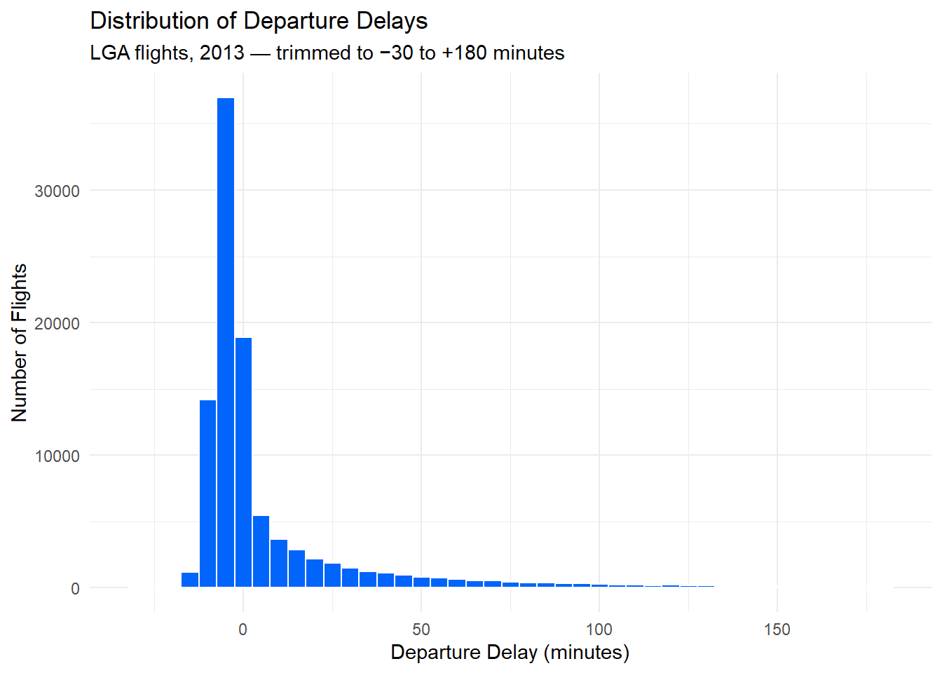

The right skew is unmistakable. The bulk of flights cluster just below zero, and a long tail of severe delays extends to the right — the same pattern the mean-vs-median comparison in the previous chapter quantified numerically.

11.5.2 Departure Delay vs. Arrival Delay

The strong correlation between departure and arrival delay is easier to see as a scatterplot than as a single number:

delay_pairs <- dbGetQuery(con, "
  SELECT dep_delay, arr_delay
  FROM flights
  WHERE dep_delay IS NOT NULL
    AND arr_delay IS NOT NULL
    AND dep_delay BETWEEN -30 AND 120
    AND arr_delay BETWEEN -60 AND 120
")

ggplot(delay_pairs, aes(x = dep_delay, y = arr_delay)) +
  geom_point(alpha = 0.05, color = "#0165fc") +
  geom_smooth(method = "lm", color = "firebrick", se = FALSE) +
  labs(
    title = "Departure Delay vs. Arrival Delay",
    subtitle = "Each point is one flight; regression line overlaid",
    x = "Departure Delay (minutes)",
    y = "Arrival Delay (minutes)"
  ) +
  theme_minimal()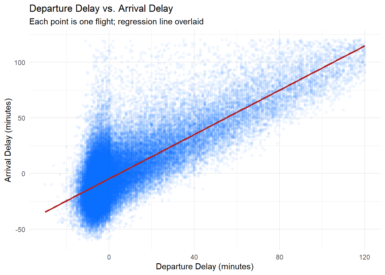

The regression line runs nearly through the origin with a slope close to 1: a one-minute departure delay corresponds to roughly one minute of arrival delay. The transparency (alpha = 0.05) reveals where the mass of flights lies despite over 100,000 overlapping points.

11.5.3 Mean Delay by Carrier

A horizontal bar chart makes carrier comparisons easy to read:

ggplot(delays_by_carrier, aes(x = mean_delay, y = reorder(name, mean_delay))) +
  geom_col(fill = "#0165fc") +
  labs(
    title = "Mean Departure Delay by Carrier",
    subtitle = "LGA flights, 2013",
    x = "Mean Departure Delay (minutes)",
    y = NULL
  ) +
  theme_minimal()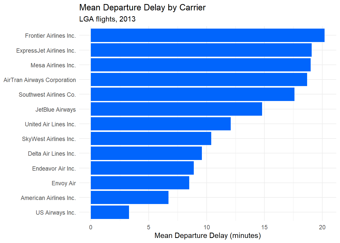

reorder(name, mean_delay) sorts the bars by delay value rather than alphabetically, making the ranking immediately visible.

11.6 Parameterized Queries

When a query needs to incorporate a value from R, the instinct is to paste it directly into the query string:

# Do not do this
carrier_code <- "AA"
dbGetQuery(con, paste0("SELECT * FROM flights WHERE carrier = '", carrier_code, "'"))

This is unsafe. If carrier_code came from user input and contained something like '; DROP TABLE flights; --, the database would execute that injected SQL. The correct approach is a parameterized query, which passes values separately from the query text so the database treats them as data, never as SQL.

DBI supports parameterized queries through the params argument. Placeholders in the query string are written as $1, $2, and so on (for PostgreSQL):

carrier_code <- "AA"

aa_flights <- dbGetQuery(
  con,
  "SELECT flight, dep_delay, arr_delay, dest
   FROM flights
   WHERE carrier = $1
     AND dep_delay IS NOT NULL
   ORDER BY dep_delay DESC",
  params = list(carrier_code)
)

head(aa_flights)

  flight dep_delay arr_delay dest
1   2019       803       802  STL
2   2437       660       648  MIA
3    731       613       598  DFW
4    753       533       499  DFW
5    731       504       493  DFW
6    745       502       495  DFW

The value of carrier_code is sent to the database separately. No matter what string is in carrier_code, it is treated as a literal value to compare against the carrier column, not as SQL to execute. Multiple parameters follow the same pattern: add more $n placeholders and extend the params list.

Always use parameterized queries whenever a query incorporates a value that originates from outside your own code, including user input, configuration files, or other data sources. The params argument is the right tool in DBI.

11.7 Closing the Connection

A database connection holds resources on both the R side and the database server side. Close it explicitly when you are done:

dbDisconnect(con)

In a script that opens a connection at the top and closes it at the bottom, it is good practice to use on.exit() to ensure the connection closes even if an error occurs partway through:

con <- dbConnect(Postgres(), host = "localhost", port = 5433,
                 dbname = "nycflights", user = "postgres", password = "postgres")
on.exit(dbDisconnect(con), add = TRUE)

# ... rest of your analysis ...

on.exit(..., add = TRUE) schedules dbDisconnect(con) to run when the surrounding function or script exits, regardless of whether it exits normally or with an error.

11.8 Exercises

11.8.1 Reflection

1. What is the relationship between the DBI package and driver packages like RPostgres? Why is this two-layer design useful?

2. Explain what is wrong with building a query string using paste0() to insert a user-supplied value. What does a parameterized query do differently, and why does it prevent SQL injection?

11.8.2 Coding

3. Connect to the nycflights database and use dbListFields() to inspect the columns of the weather table. Then write a dbGetQuery() call that retrieves the average temperature (temp) and average wind speed (wind_speed) for each month. Store the result in a data frame and print it.

4. Using dbGetQuery(), retrieve the number of flights per destination (dest) from the flights table. Then use ggplot2 to create a bar chart of the top 15 destinations by flight count.

5. Write a parameterized query that accepts a minimum number of Oscar nominations as a parameter and returns matching actors from the actors database. (You will need to open a second connection to the actors database.) Test it with at least two different threshold values.

6. Retrieve daily average departure delay from flights (aggregate by month and day). Plot the result as a line chart with ggplot2, using month and day to construct a date on the x-axis. Describe the seasonal pattern you observe.

R Special Interest Group on Databases (R-SIG-DB), Hadley Wickham, and Kirill Müller. 2026. DBI: R Database Interface. https://dbi.r-dbi.org.

Wickham, Hadley. 2016. Ggplot2: Elegant Graphics for Data Analysis. Springer-Verlag New York. https://ggplot2.tidyverse.org.